SVM: How does Support Vector Machine work?

This is a series where I answer the questions my tutoring students really ask – the ones textbooks tend to skip. I teach machine learning, deep learning, statistics, and math to learners of all levels.

---

The question. A student prepping for her qualifying exam waved her lecture notes at me: “My perceptron homework already converged to a perfectly good separating line, so what is the SVM optimizing that the perceptron is not? Everyone says ‘maximum margin’ and ‘support vectors’ – and then the dual pops out alphas from nowhere. How do you actually get w1, w2, b, and those alphas without a solver?”

The answer is beautifully concrete: the SVM paves the widest possible street between the two classes, and the few points touching the gutters hand you three linear equations on a plate. Let us do one street by hand.

Why isn’t any separating line good enough?

Look at the three points below – two positives (+) and one negative (o):

 3 |
 2 |
 1 |                  +        + = x1 = (3, 1)
 0 |    o                      o = x3 = (1, 0)
-1 |                  +        + = x2 = (3, -1)
-2 |
    +-----------------------------|  x1
         1      2      3
      x1 = 1 x1 = 2 x1 = 3

Infinitely many lines separate these points. A perceptron would happily hand you any one of them. An SVM asks a better question: which line would we least regret if a new point showed up near the edge?

Its answer: pave the widest street between the two classes and drive down the center line.

• The two edges of the street are the gutters.
• The points touching the gutters are the support vectors – move or delete anything else and the boundary does not budge.

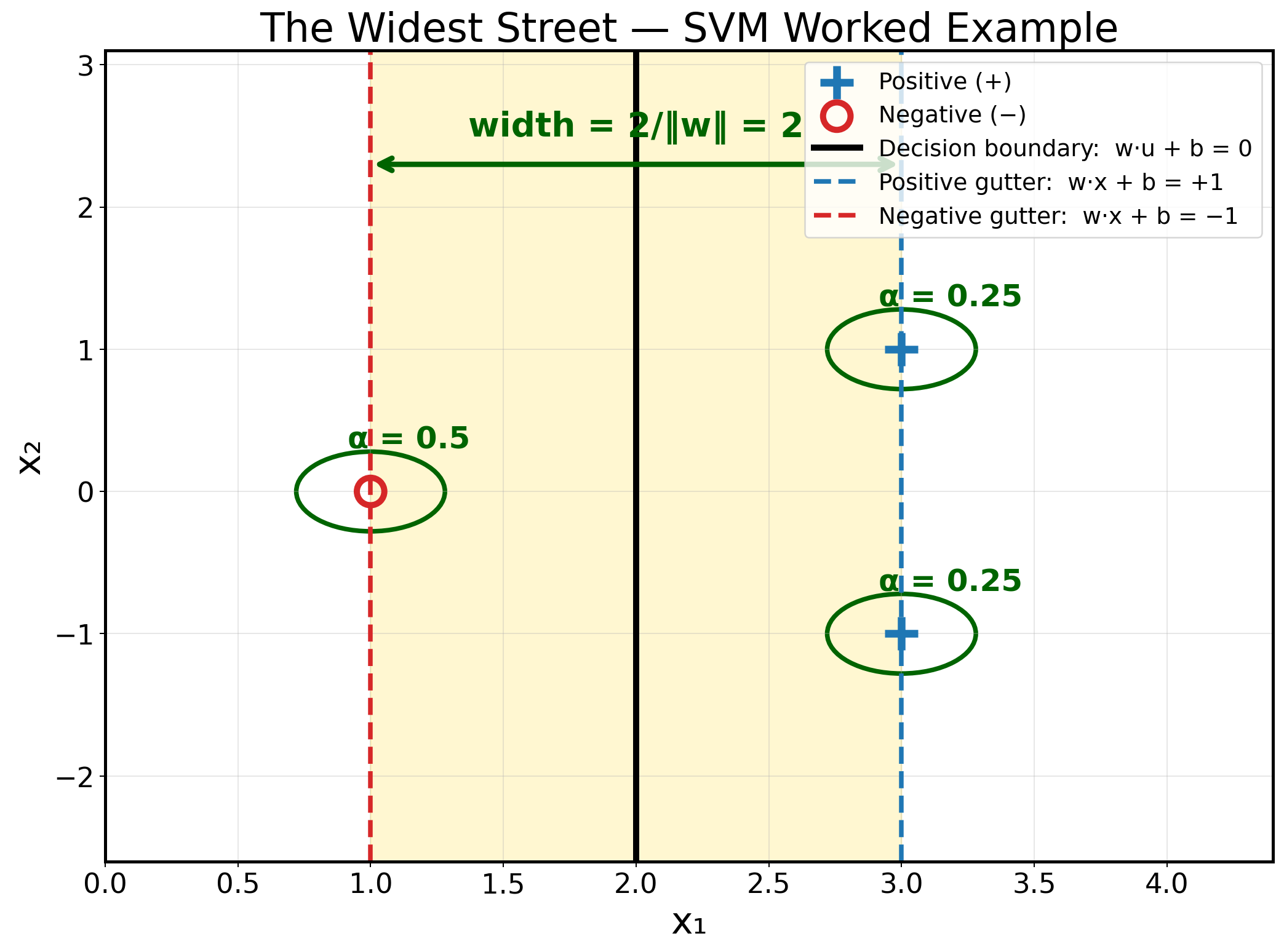
Key idea. Among all separating boundaries, the maximum-margin one generalizes best. That single design choice is what makes an SVM an SVM.

What exactly is the machine optimizing?

The decision rule. Classify an unknown point u by which side of the boundary it lands on: if w.u + b comes out zero or positive, predict positive; otherwise predict negative. The vector w is perpendicular to the boundary – it points across the street.

The constraints. Demand a safety margin of 1 on each side. With labels y_i in {+1, -1}, both sides collapse into one compact inequality that must hold for every training point:

y_i (w . x_i + b)  is at least 1     for every training point i

And here is the hand-solving gold: points on the gutters satisfy it with equality.

Why is the street width 2/||w||? Take x+ on the positive gutter and x- on the negative gutter. Their gutter equations say w.x+ + b = +1 and w.x- + b = -1, so subtracting gives w.(x+ - x-) = 2. Now project the gap between the two points onto the unit normal w/||w||: the projection is exactly the street width, and it equals 2/||w||.

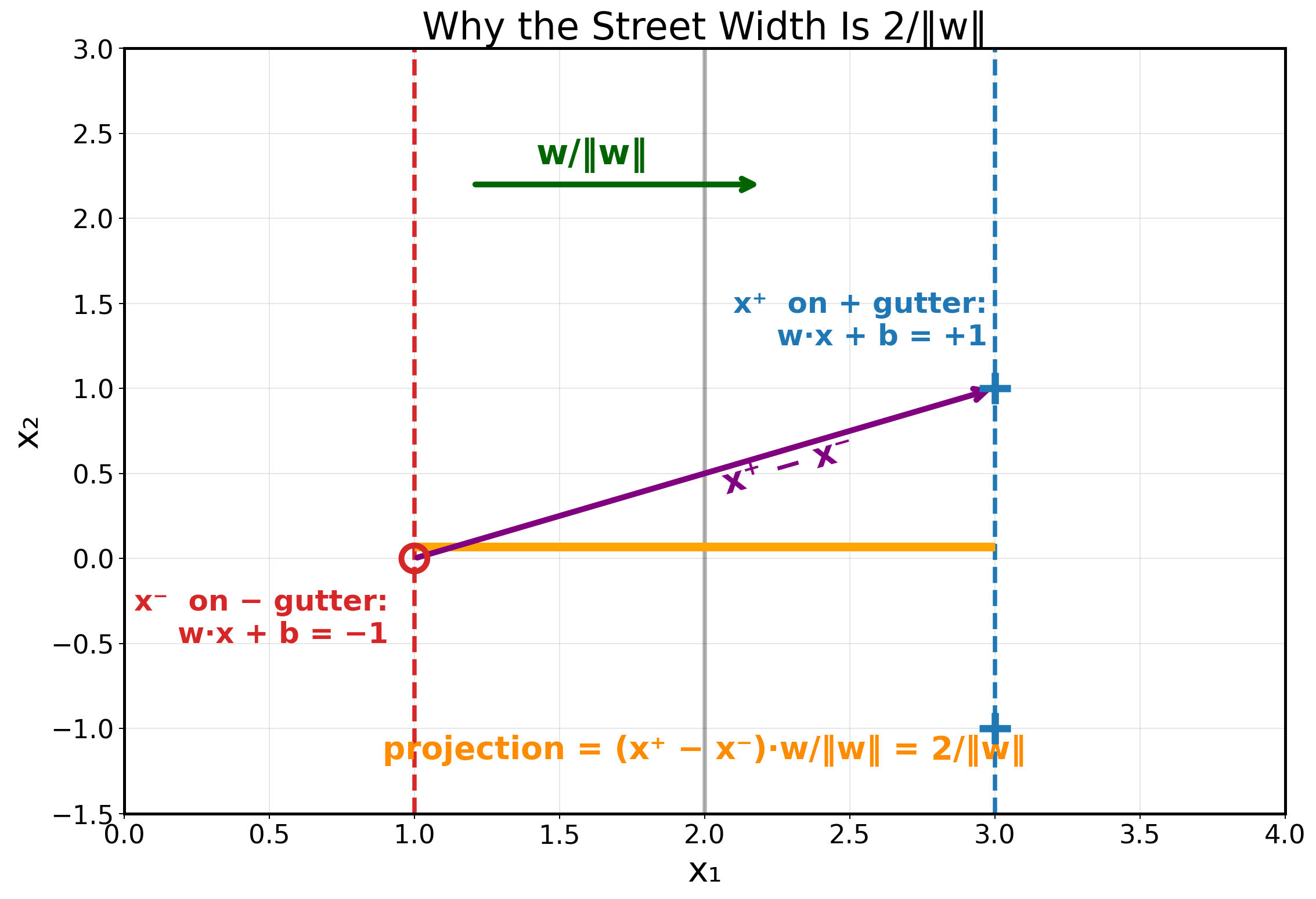
So maximizing the width means minimizing ||w||, and for a clean derivative we minimize (¹⁄₂)||w||^2 subject to the constraint above.

How do we compute w1, w2, and b by hand?

Take the worked example: x1 = (3, 1) with y1 = +1, x2 = (3, -1) with y2 = +1, and x3 = (1, 0) with y3 = -1. From the picture, the widest street runs vertically – gutters at x1 = 3 and x1 = 1 – and all three points touch a gutter. So all three are support vectors, each obeying the gutter equality y_i (w . x_i + b) = 1. That gives three equations in the three unknowns w1, w2, b, and they solve by simple subtraction:

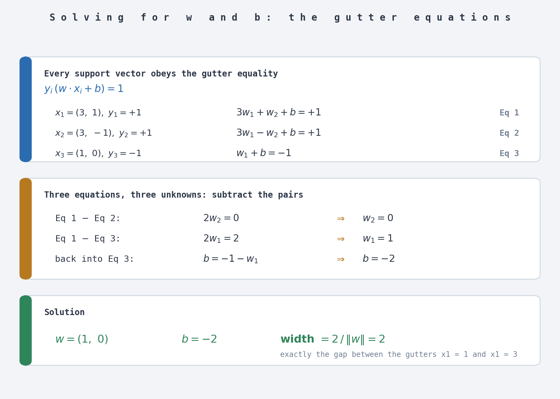
The result: w = (1, 0) and b = -2, so the decision rule is just h(u) = u1 - 2, positive whenever u1 is 2 or more. Sanity check: the width is 2/||w|| = ²⁄₁ = 2, exactly the gap between the gutters x1 = 1 and x1 = 3.

How do we get the alphas?

The optimizer does not solve for w directly – it solves for one multiplier alpha_i per constraint via Lagrange. Setting the derivatives of the Lagrangian to zero yields two identities worth memorizing:

w = sum_i alpha_i y_i x_i          w is a blend of the support vectors
sum_i alpha_i y_i = 0              the alphas must balance

The dual problem then maximizes sum_i alpha_i - (¹⁄₂) sum_i sum_j alpha_i alpha_j y_i y_j (x_i . x_j) subject to every alpha_i being zero or positive, and most alpha_i come out zero. Non-zero alpha means support vector. That is the formal meaning of “only the gutter points matter.”

For our example we already know w = (1, 0), so the first identity is one vector equation in three unknowns, and the sum rule supplies the missing constraint:

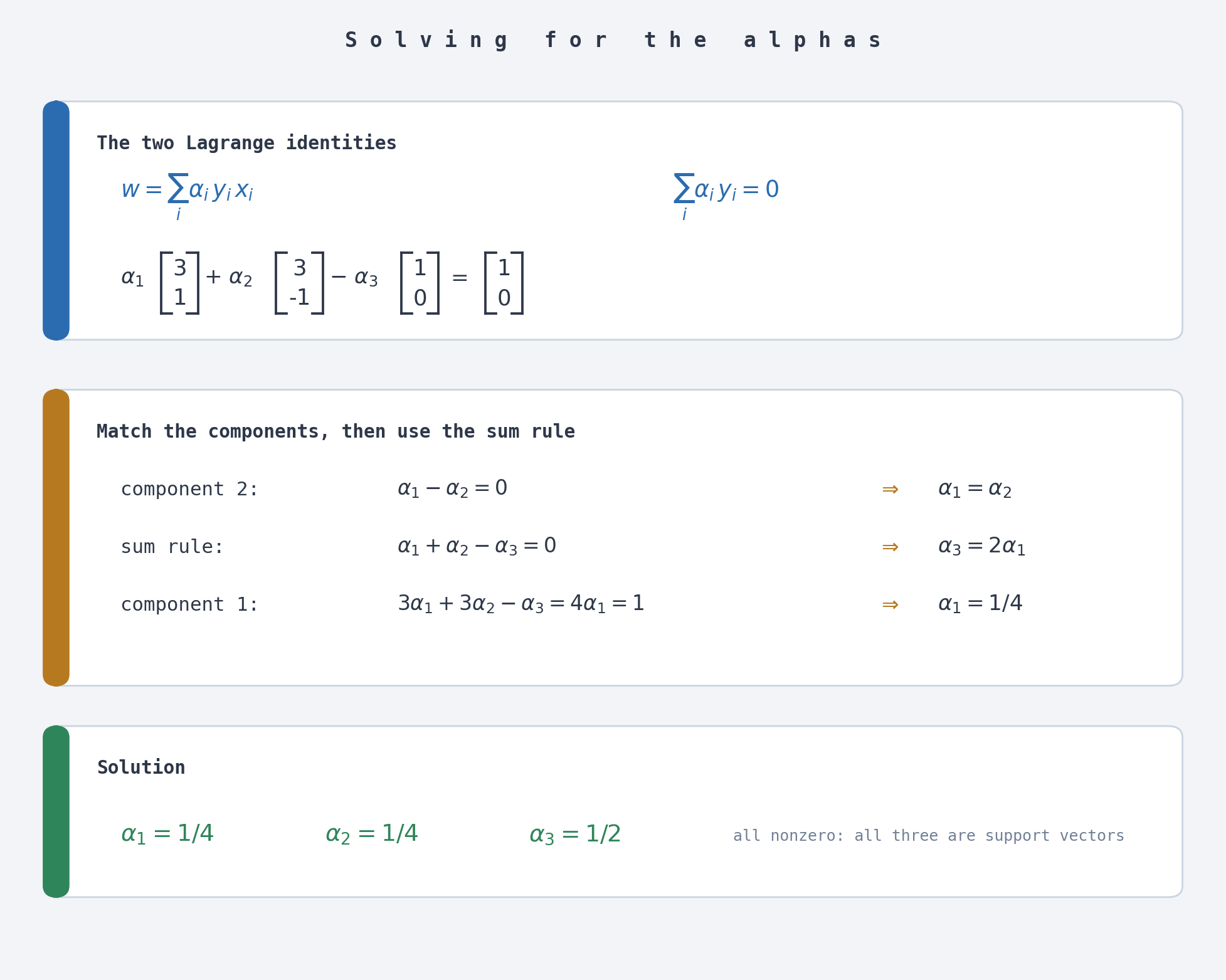
The result: alpha_1 = ¹⁄₄, alpha_2 = ¹⁄₄, alpha_3 = ¹⁄₂. Notice the lone negative point carries the biggest alpha: it is one against two, so it has to push harder. Compare with the first figure – the green rings scale with each point’s alpha.

How do we classify a new point?

Just plug it into the rule we already solved. For u = (5, 2):

h(u) = w . u + b = 1*5 + 0*2 - 2 = 3

The score is 3, which is positive, so u lands on the positive side of the street and we predict positive.

No retraining. And a new point that lands far from the street, say a negative point at (0, 6)? It gets alpha = 0 and changes nothing – the boundary stays exactly where it is.

Can we verify this in 30 lines of Python?

Yes – this cell solves the same linear systems and cross-checks against scikit-learn:

import numpy as np
from sklearn.svm import SVC

X = np.array([[3, 1], [3, -1], [1, 0]])
y = np.array([+1, +1, -1])

# Step 1: solve the gutter equalities  y_i (w . x_i + b) = 1
A = np.column_stack([X, np.ones(3)])
w1, w2, b = np.linalg.solve(A, y.astype(float))
print(f"w = ({w1:.2f}, {w2:.2f}), b = {b:.2f}, width = {2/np.linalg.norm(w1):.2f}")
# prints  w = (1.00, 0.00), b = -2.00, width = 2.00

# Step 2: alphas from  w = sum alpha_i y_i x_i  and  sum alpha_i y_i = 0
M = np.vstack([(y[:, None] * X).T, y])
print("alphas =", np.round(np.linalg.solve(M, [w1, w2, 0.0]), 4))
# prints  alphas = [0.25 0.25 0.5 ]

# Cross-check with a real SVM
clf = SVC(kernel="linear", C=1e6).fit(X, y)
print(clf.coef_, clf.intercept_, clf.predict([[5, 2]]))
# prints  [[1. 0.]] [-2.] [+1]

By hand and by library, same answer.

What if no straight line works – how does the kernel trick rescue us?

Here is the beautiful structural fact: both the dual objective and the final classifier touch the data only through dot products x_i . x_j. So we are free to swap every input for a transformed one, x becomes phi(x), as long as we can still compute dot products there. That is a kernel: K(u, v) = phi(u) . phi(v). We never compute phi itself – only K – even if phi lands in a space with millions (or infinitely many) dimensions.

Take six points on a line: negatives at x = -3, -2, +2, +3 and positives at x = -1, +1:

   o     o     +     +     o     o
  -3    -2    -1     1     2     3
   |-----|-----|-----|-----|-----|   x
          no single cut works here

No threshold on x separates them – a plain SVM fails. Now lift every point with phi(x) = (x, x^2). The positives drop to height 1, the negatives rise to heights 4 and 9, and a flat horizontal boundary at x^2 = 2 splits them perfectly:

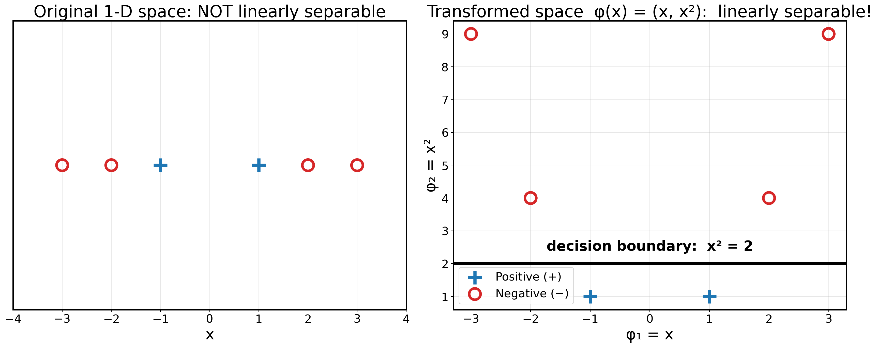
In the original space the boundary looks like a parabola (two thresholds at x = -sqrt(2) and x = +sqrt(2)); in the transformed space it is just a straight gutter – maximum margin and all. And we never had to name phi: a polynomial-style kernel such as K(u, v) = (u.v + 1)^2 already produces the x^2 term implicitly.

Quick self-check

Q: A new negative point appears at (0, 0) – inside its class region. What is its alpha?

Answer: 0. It is safely on its own side of the gutter, so it is not a support vector. Non-support points never get weight.

Q: The support vector (3, 1) slides out to (4, 1). Does its alpha grow or shrink?

Answer: it shrinks. The street gets wider (from 2 to 3), so ||w|| = 2/width shrinks from 1 to ²⁄₃, and since w = sum_i alpha_i y_i x_i, the alphas shrink with it. Wider street, smaller alphas.

One-page summary

Concept	Formula or fact
Decision rule	h(u) = sign(w . u + b)
Constraint, all points	y_i (w . x_i + b) - 1 is at least 0
Gutter equality, support vectors	y_i (w . x_i + b) = 1
Street width	2 /
Key identities	w = sum_i alpha_i y_i x_i and sum_i alpha_i y_i = 0
Dual objective	maximize sum_i alpha_i - (1⁄2) sum_i sum_j alpha_i alpha_j y_i y_j (x_i . x_j)
Support vectors	points with alpha_i above zero; they alone define the boundary
Kernel trick	replace u.v by K(u, v) = phi(u) . phi(v)

Hand-solving recipe for exams: 1. draw the points, 2. find the widest street and its support vectors, 3. solve y_i (w . x_i + b) = 1 for w and b, 4. solve w = sum alpha_i y_i x_i together with sum alpha_i y_i = 0 for the alphas, 5. everything off the gutters gets alpha = 0.

---

The arithmetic and diagrams in this article are adapted from the teaching notebooks I use with my students, where every weight and alpha is computed by hand before any library is allowed.

References

1. Winston, P. H. (2010). “Learning: Support Vector Machines.” 6.034 Artificial Intelligence, Lecture 16, MIT OpenCourseWare, Fall 2010. video
2. Seifter, M. (2010). “Mega-Recitation 5: Support Vector Machines.” 6.034 Artificial Intelligence, MIT OpenCourseWare, Fall 2010. video
3. Winston, P. H. “SVM Practice Exercises.” 6.034 Artificial Intelligence handout, MIT. PDF

I tutor machine learning, deep learning, statistics, and math. If SVMs – or anything else – are not clicking for you, you can find me on Wyzant.