Gated Memory: How do LSTM, GRU, and KDA remember the same token differently?

This is a series where I answer the questions my tutoring students really ask – the ones textbooks tend to skip. I teach machine learning, deep learning, statistics, and math to graduate students and working engineers.

The question. After we ran an LSTM against a GRU, and then an LSTM against the Kimi Delta Network, a student put the obvious follow-up on the table: “Can we see all three side by side? If the same token arrives with the same memory, what does each architecture do to the numbers?”

That is exactly the right way to ask it, because the difference between these models only becomes visible in arithmetic. So let’s take the sentence “your journey starts with one step” and watch all three models process a single moment: the instant the token “journey” arrives right after “your”. To keep every number visible, the memory state gets just three dimensions. One detail matters throughout: gates act per dimension, so every gate below is a vector of three numbers, one for each dimension of the memory state, and each dimension makes its own keep-or-add decision.

Want to move the dials yourself? The companion interactive visualization lets you drag any slider and watch every number below recompute live: LSTM, GRU, and KDA, one interactive step.

The setup. The token “journey” arrives as x1 = [0.55, 0.87, 0.66], and yesterday’s memory, left over from “your”, is s0 = [0.80, 0.50, 0.30]. Every gate value below is a realistic sigmoid or tanh output:

shared    s0    = [0.80, 0.50, 0.30]    yesterday's memory (LSTM and GRU)
shared    f     = [0.90, 0.50, 0.10]    forget gate (LSTM, shared with GRU)
LSTM      i     = [0.10, 0.30, 0.80]    input gate
LSTM      o     = [1.00, 0.50, 0.20]    output gate
LSTM      a1    = [0.60, -0.40, 0.90]   candidate (tanh output)
GRU       r     = [1.00, 0.50, 0.00]    reset gate
GRU       a1~   = [0.55, -0.20, 0.30]   candidate (built from r * s0)
KDA       s     = 0.40                  strength of "your" stored in step 1 (beta1 * v = 0.8 * 0.5)
KDA       alpha = [0.50, 0.90, 1.00]    per-channel decay, step 2
KDA       beta  = 1.00                  write strength, step 2
KDA       v     = [0.00, 0.80, 0.20]    value written by "journey"
KDA       k = [0, 1, 0],  q = [0, 1, 0] key and query for "journey"

What the dials mean

Before any arithmetic, here is the vocabulary of each model, side by side:

The short version: the LSTM’s forget and input gates are independent, so keeping and adding are separate decisions. The GRU ties them together, so the write dial is forced to be whatever the keep dial leaves behind. KDA replaces dials with a dictionary: the key says which slot to erase and write, the value is what gets written, and the query says which slot to read.

The three update rules

All three models solve the same problem: keep some of the old memory, add some new content, and produce a readout. They differ only in how much freedom each step is given.

It helps to read these as one skeleton spoken in three dialects. The memory s0 corresponds to the matrix S. The forget gate f corresponds to Diag(alpha). The input term i * a1 corresponds to the write beta * v * k^T. And the readout h1 corresponds to S * q. What changes from line to line is how the parts are tied together: the LSTM leaves keep and add independent, the GRU forces them to sum to one, and KDA addresses every write and every read to a specific key.

Step by step: keep, add, read

Here is the full computation for all three models, with every intermediate vector and matrix shown:

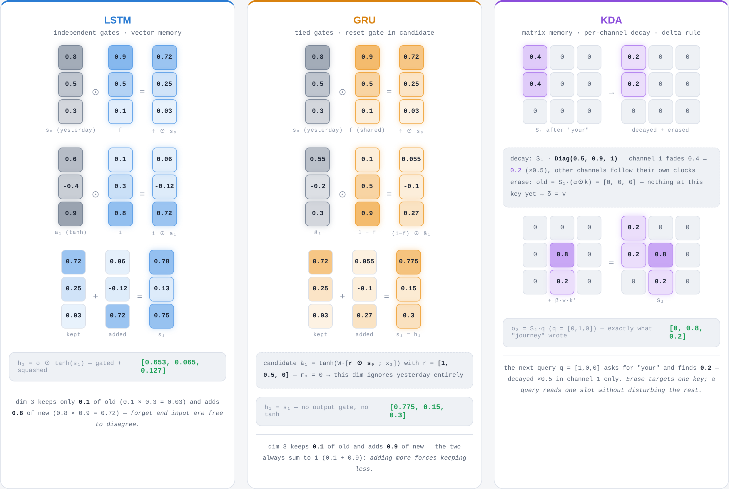
For the LSTM, watch the third dimension. The model keeps only 0.10 x 0.30 = 0.03 of the old value and simultaneously writes 0.80 x 0.90 = 0.72 of the new one. Forget and input are free to disagree, and here they do. Then a separate decision is made about exposure: tanh squashes 0.75 down to 0.635, and the output gate shows only 20% of it, so the outside world sees 0.127.

For the GRU, the keep side is identical because the forget gate is shared, but the write side is forced to be 1 - f. In dimension 3 the GRU keeps 0.10 of the old and adds 0.90 of the new, and the two always sum to one: adding more forces keeping less. Notice also that the candidate is built from r * s0 with r3 = 0, which makes dimension 3 completely blind to yesterday before it even gets a say. With no output gate and no tanh, the raw state h1 = s1 = [0.775, 0.15, 0.30] is exposed.

For KDA, the memory is a 3 x 3 matrix and the word “your” sits in column 1 with strength 0.4 from step 1. The decay-plus-erase matrix fades channel 1 from 0.4 to 0.2, multiplied by alpha1 = 0.5, while the other channels follow their own clocks. Because nothing was stored at the key k = [0, 1, 0] before, the delta rule’s correction is simply delta = v, and “journey” writes [0.00, 0.80, 0.20] into that slot. Reading with q = [0, 1, 0] returns exactly what “journey” wrote, and the payoff comes on the next step: a query q = [1, 0, 0] asking for “your” finds 0.2, faded only in channel 1, with the rest of the matrix untouched. The erase targeted one key, and the query reads one slot without disturbing anything else. That is what it means for memory to be a dictionary rather than a dial.

Same step, three behaviors: focus on dimension 3

Dimension 3 held 0.30 yesterday. Here is what each model keeps of it, what it adds, and what it shows:

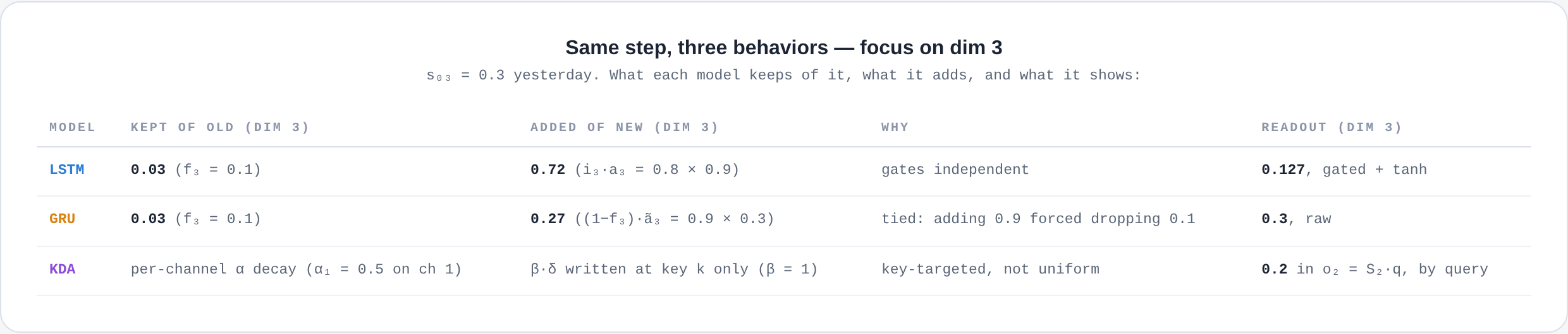
The table is the whole argument in one row per model: the LSTM’s gates act independently, the GRU’s are tied so that adding 0.90 forced dropping 0.90, and KDA is key-targeted rather than uniform.

Takeaways

The LSTM gets two free dials, one for keeping and one for adding, and then chooses what to show through a separate output gate. The GRU collapses keeping and adding into a single dial, so every bit of new content is paid for with forgotten old content, and it shows everything it has. KDA keeps per-channel, writes by key, and reads by query: memory stops being a dial you turn and becomes a dictionary you update and look things up in.

This post is the static companion to the interactive visualization, in which every slider recomputes every number live; the values above are its default settings. If you have not read them yet, the two predecessor posts in this series walk the same ground in pairs: an LSTM against a GRU on a day of temperature forecasting, and an LSTM against the Kimi Delta Network on this same sentence.