Loss Functions: Which to use?
This is a series where I answer the questions my tutoring students really ask – the ones textbooks tend to skip. I teach machine learning, deep learning, statistics, and math to learners of all levels.
The question. “I picked MSE for my regression and one glitched row wrecked the whole fit. My classifier runs softmax + cross-entropy because that is what every tutorial does. But nobody ever told me why – or what happens if I pick wrong. Which loss should I actually use?”
The loss function is the rulebook you hand the optimizer: it decides what counts as a mistake and how badly each mistake is punished. Gradient descent never argues with the rulebook; it just follows it, faithfully, into whatever ditch the rulebook points at. Choosing the loss is choosing the target. Here is the whole menu – MSE, MAE, Huber, hinge, BCE, softmax + CCE – each with the same kind of hand arithmetic we do in the tutoring session.
Regression, round 1: MSE versus MAE
The two formulas everyone knows:
MSE = (1/n) * sum_i (y_i - yhat_i)^2
MAE = (1/n) * sum_i |y_i - yhat_i|
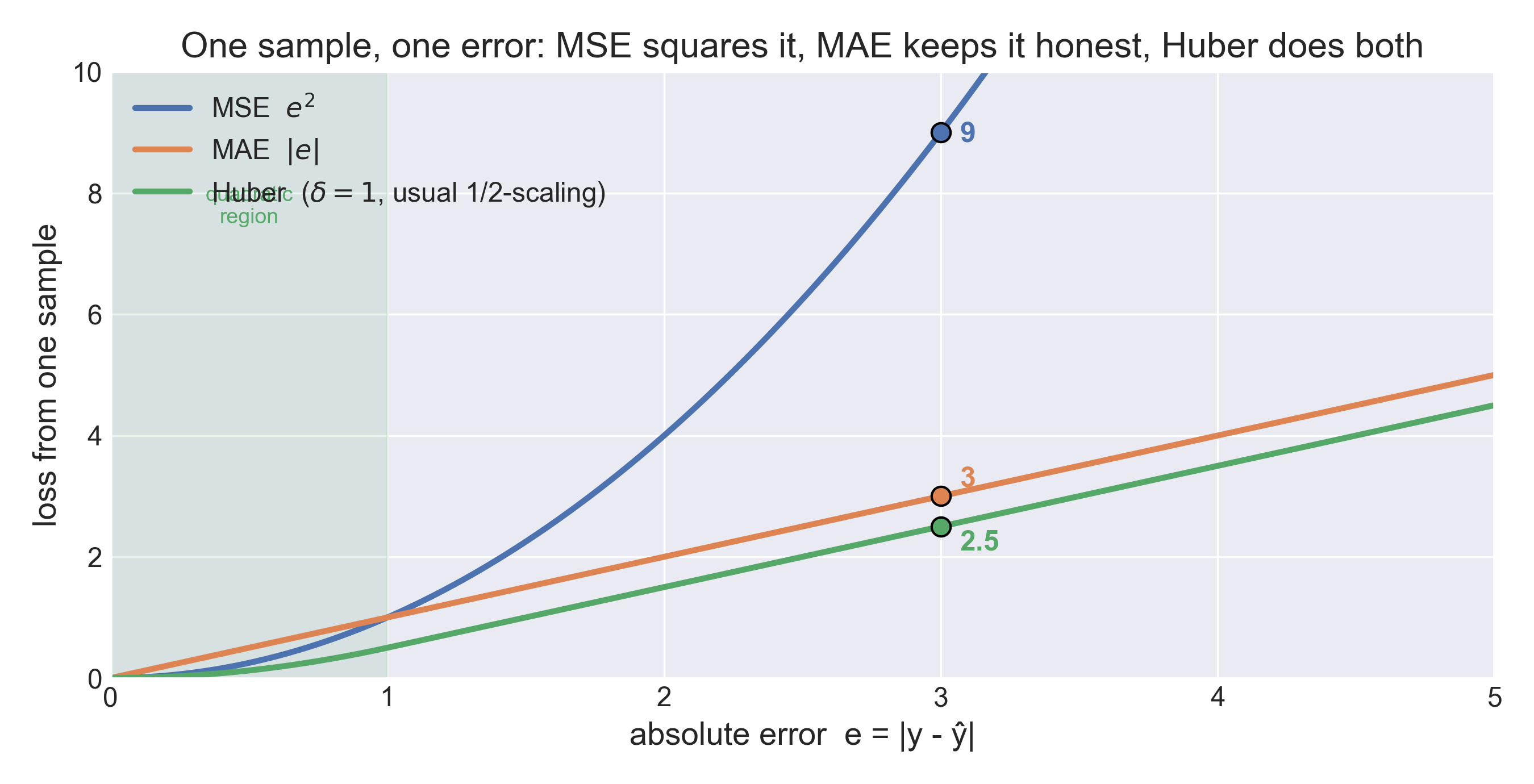
Same sum, same average – one difference: MSE bills the square of the error, MAE bills the error itself. Run one sample through both and the personality shows immediately. Take an absolute error e = 3:
MSE contribution:  e^2  = 9
MAE contribution:  |e|  = 3
Now watch how the bill scales as the error grows:
error e     1    2    3     5
MSE         1    4    9    25
MAE         1    2    3     5
Up to e = 1 they agree (1^2 = 1 – the crossing point in the figure). Past that, MSE’s bill grows quadratically while MAE’s grows linearly. That single fact explains every difference in behavior: the gradient MSE hands back is proportional to 2e, so a sample sitting 5 units away pushes with slope 10, while MAE pushes with a constant slope of +/-1 no matter what.
The outlier test: who actually minimizes each bill?
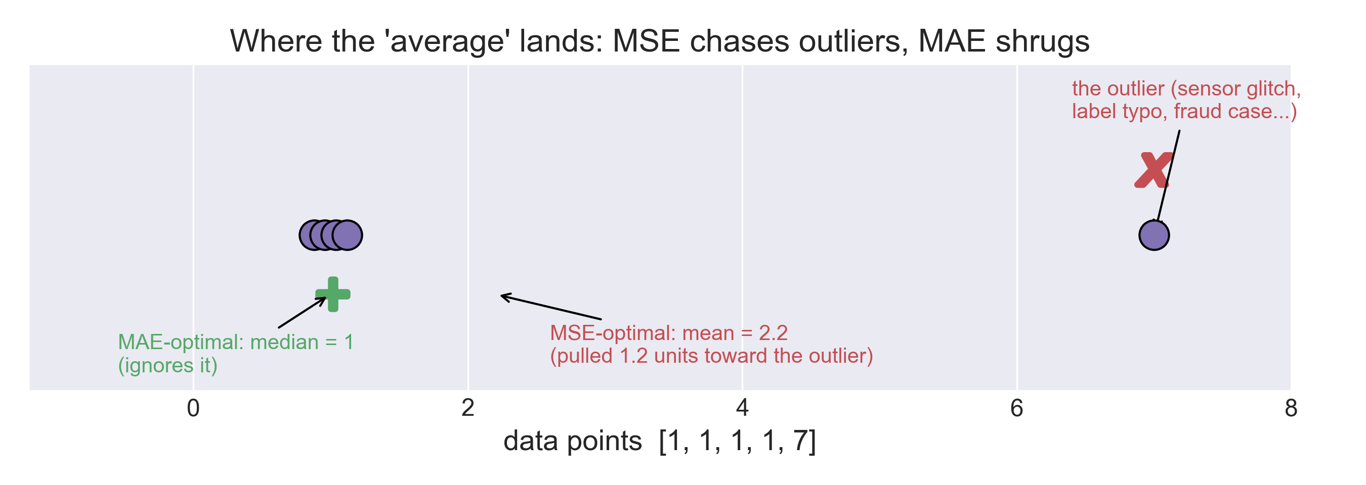
“Robust to outliers” sounds like marketing language until you compute it. Five measurements, four of them 1 and one glitch at 7 – a temperature sensor spike, a mistyped label, a fraudulent transaction. Your model predicts one constant c. MSE wants the c minimizing sum (p_i - c)^2; MAE wants the c minimizing sum |p_i - c|. Two candidates:
            MSE: SSE          MAE
c = 2.2:    28.8   <-- MSE winner     1.92
c = 1.0:    36.0                       1.20   <-- MAE winner
MSE’s best answer is the mean, 2.2 – dragged 1.2 units toward the outlier, wrong for four of the five points. MAE’s best answer is the median, 1.0 – it ignores the glitch completely. That is the entire robustness story in one row of numbers: MSE’s optimum is the mean, MAE’s optimum is the median.
Huber loss: the truce
MSE is great on clean data – smooth, differentiable, statistically optimal when the noise really is Gaussian. MAE is great on dirty data – but its constant slope is noisy near the minimum and its corner at zero is not differentiable. Huber loss takes the good half of each, with a switch point d:
L_d(r) = 0.5 * r^2            if |r| <= d
       = d * (|r| - 0.5 * d)  if |r| >  d
With d = 1: a small error of 0.5 costs 0.5 * 0.5^2 = 0.125 – pure MSE behavior. A big error of 3 costs 1 * (3 - 0.5) = 2.5 – pure MAE behavior: linear, so outliers cannot hold the model hostage. The two branches meet exactly at |r| = d (both give 0.5 * d^2), so the curve has no corner and the gradient exists everywhere. Look at the green curve above: quadratic in the shaded region, straight lines outside it. It is the default I recommend when a student says “my data is mostly clean but I trust it maybe ninety percent.”
Classification: why MSE quietly fails
So why does nobody use MSE on a classifier? Take the sigmoid output yhat = sigmoid(z) and MSE. When the model is very wrong – say yhat close to 0 for a true positive – you would expect a loud alarm. Instead the MSE gradient is proportional to (yhat - y) * yhat * (1 - yhat), and that middle yhat * (1 - yhat) factor is nearly zero when the sigmoid saturates. Confidently wrong produces silence: a plateau where learning crawls. Cross-entropy cancels that factor exactly. It was designed, in effect, to be the sound partner of the sigmoid.
Cross-entropy: the price of surprise
Here p is the true distribution and q the predicted one:
H(p, q) = -sum_i p(i) * log q(i)
For classification the truth is a one-hot vector – p(i) = 1 on the true class, 0 elsewhere – so the sum collapses to a single term:
H(p, q) = -log q(y_true)
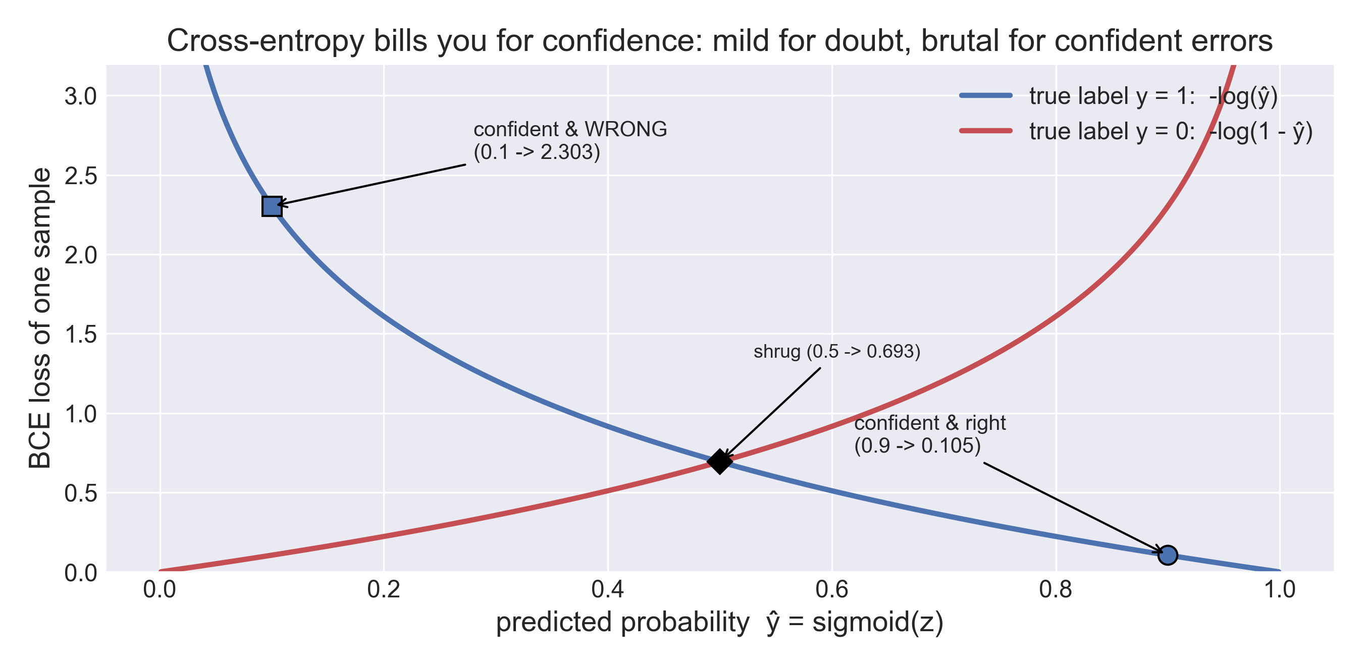
Read that as a surprise tax: you pay minus the log of whatever probability you handed the truth. The price list:
you said      0.9      0.5      0.1
loss       0.105    0.693    2.303
Doubt is taxed gently; confident error is taxed brutally – -log(0.1) is 22 times -log(0.9). This is not an aesthetic choice: cross-entropy is negative log-likelihood, so minimizing it is maximum likelihood estimation, the same principle that makes MSE the “right” loss for Gaussian noise.
There is also an accounting identity worth knowing (it lives in my notebook, and in every VAE lecture):
H(p, q) = H(p) + KL(p || q)
Cross-entropy = the true entropy plus the KL divergence, the extra cost of encoding p as if it were q. When p is a fixed label, H(p) is a constant, so minimizing cross-entropy and minimizing KL divergence are the same job – one word shorter, same gradient. (When p is itself learned, as inside a VAE, H(p) stops being constant and the two are not equivalent anymore – a classic exam question.)
Binary: sigmoid + BCE
For one yes/no output, the cross-entropy tax on both label values is
BCE = -(1/n) * sum_i [ y_i * log(yhat_i) + (1 - y_i) * log(1 - yhat_i) ]
Worked example, no library allowed. Logit z = 2.0, so yhat = sigmoid(2.0) = 1 / (1 + e^-2) = 0.881. If the truth is y = 1:
loss = -log(0.881) = 0.127 (mild: 88% confidence in the truth)
If the truth is y = 0 instead, the same prediction gets billed for the other branch:
loss = -log(1 - 0.881) = -log(0.119) = 2.127 (harsh: confident and wrong)
And the reward for combining them: the derivative of BCE composed with the sigmoid is simply yhat - y. One clean subtraction – no sigmoid-derivative term to vanish on you. This is why “sigmoid + BCE” is a package deal, listed together on every menu.
One more row of numbers before we move on: on 100 emails where 2 are spam, a model that always says yhat = 0.02 scores BCE about 0.09 – excellent average, completely useless detector. The loss is not broken; it is answering a different question than the one you care about. When classes are lopsided, weight the positive term or reach for focal loss – but check the confusion matrix before trusting any loss number.
Multi-class: softmax + CCE
Softmax converts raw scores into a probability distribution, and categorical cross-entropy bills the true class:
p_i  = exp(z_i) / sum_j exp(z_j)
loss = -log p_true
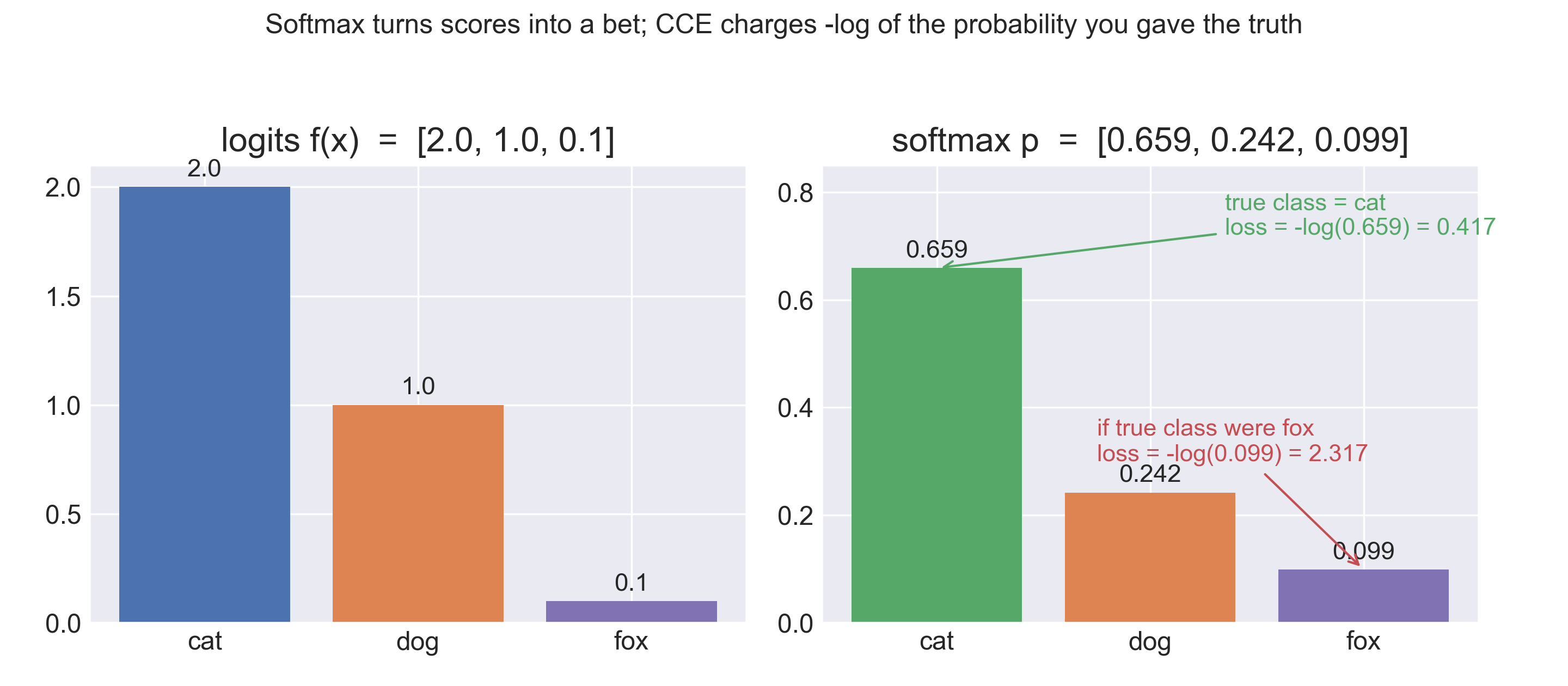
Take logits z = [2.0, 1.0, 0.1] for (cat, dog, fox) and do it by hand:
exp(z)     = [7.389, 2.718, 1.105]
sum        = 7.389 + 2.718 + 1.105 = 11.212
softmax p  = [0.659, 0.242, 0.099]
Notice the exponentials widen the gaps before normalizing: score ratios of 2:1:0.1 become probability ratios of 6.7:2.5:1. Now the bill depends on where the truth sits:
true = cat:  -log(0.659) = 0.417      the model favored the truth
true = fox:  -log(0.099) = 2.317      the model bet against it
Same prediction, six times the loss – because cross-entropy only asks one question: how much did you give the truth? And again the gradient is the beautiful one: d(loss)/d(z) = p - onehot, an “adjust your bet” signal. Softmax + CCE is why every classifier from digit recognition to GPT’s next-token prediction ends in the same two layers.
Hinge: the SVM’s margin philosophy
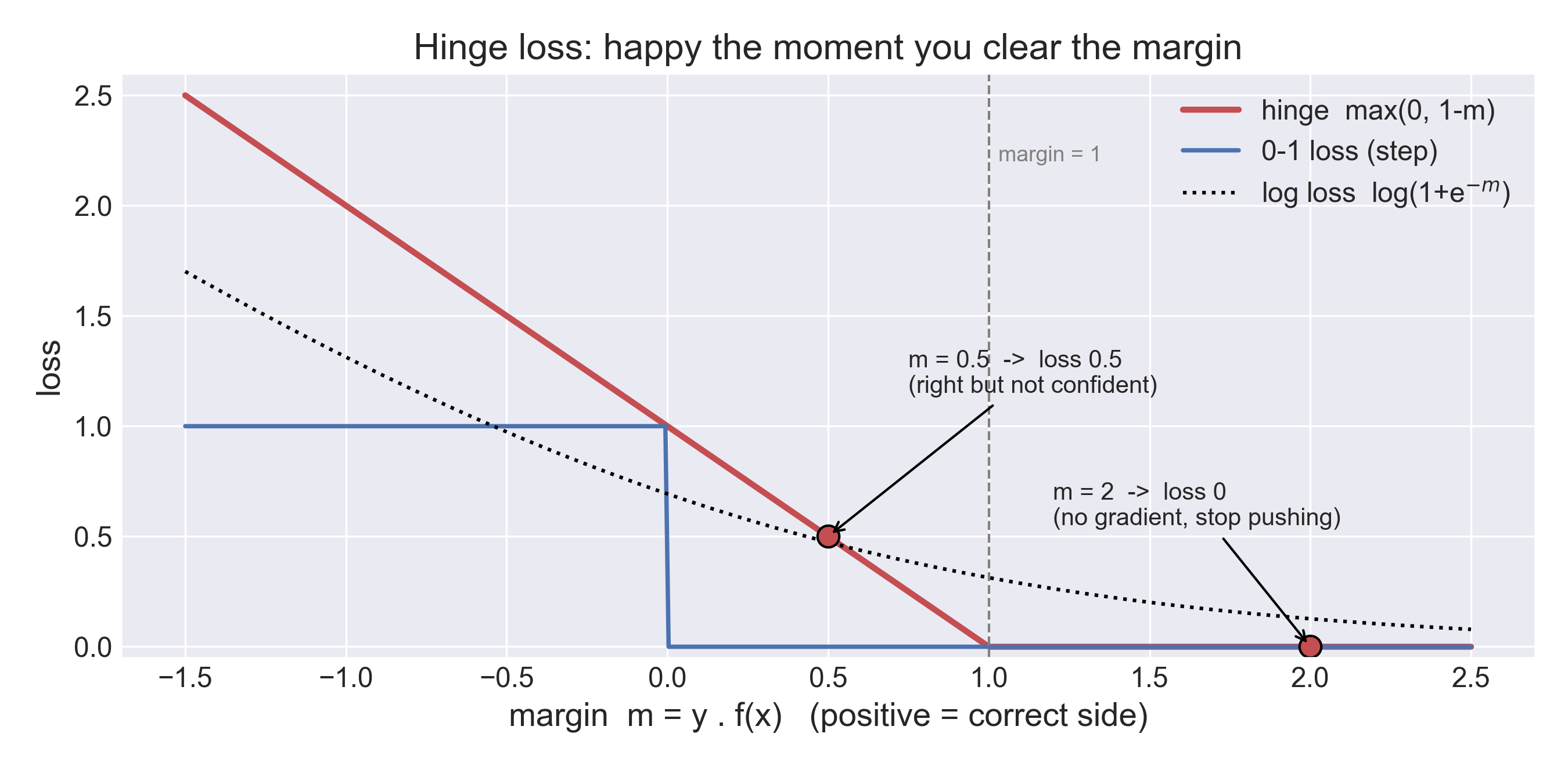
Hinge loss asks something different of a classifier. Let the margin be m = y * f(x) (positive when you are on the correct side):
L = max(0, 1 - m)
Be right and confidently right by a margin of at least 1 – then your loss is exactly zero, your gradient is zero, and the model stops pushing you:
m =  0.5:   loss = max(0, 1 - 0.5)  = 0.5     right, not confident
m =  2.0:   loss = max(0, 1 - 2.0)  = 0       done, move on
m = -0.5:   loss = max(0, 1 + 0.5)  = 1.5     wrong side
Compare with the 0-1 loss (a raw step function, no gradient) and the log loss (taxes even the confidently correct, forever). The hinge is the compromise: differentiable where it matters, indifferent once you clear the fence. That indifference is the whole SVM idea – only the support vectors, the samples within the margin, ever contribute.
So which one should you use?
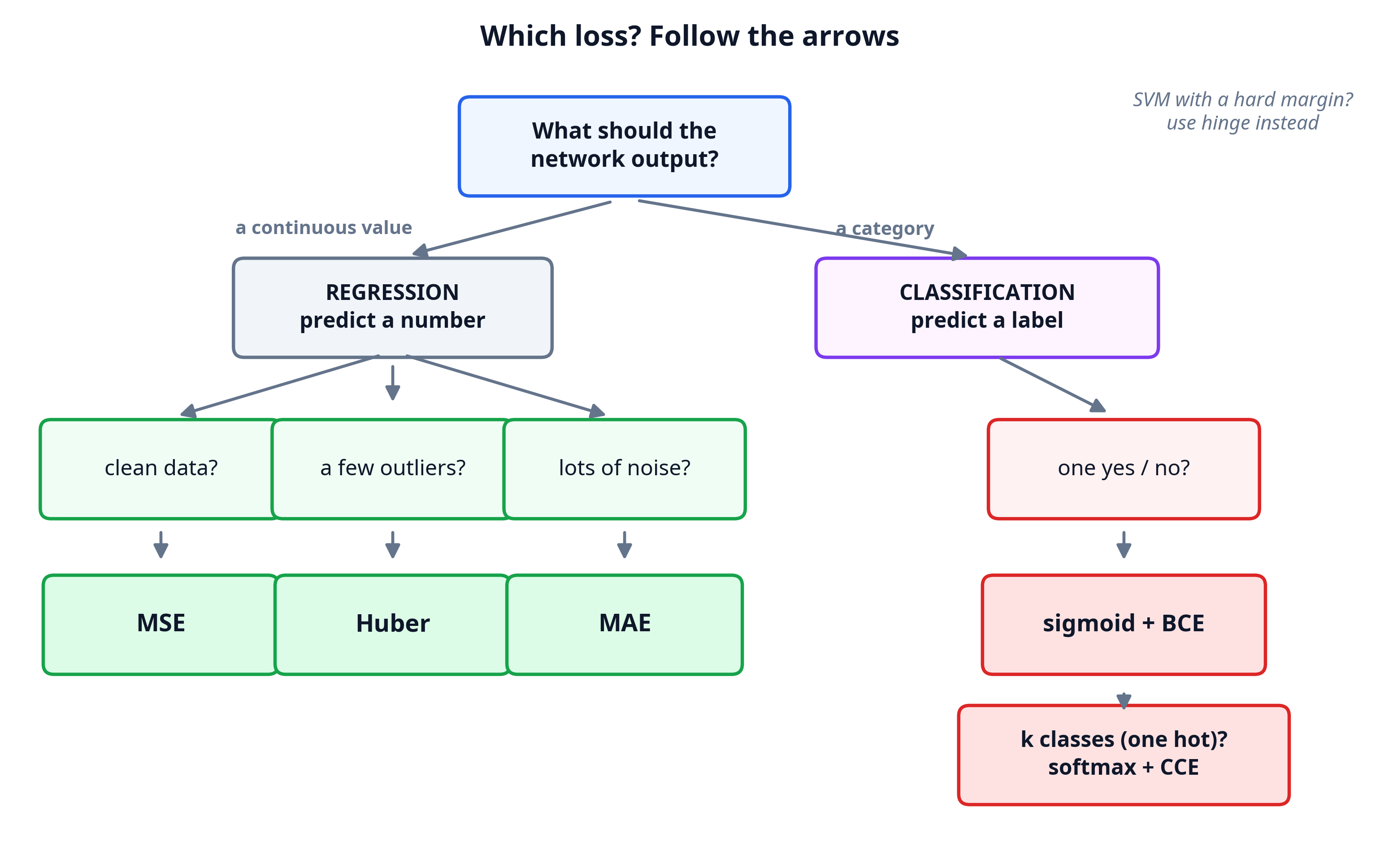
The pragmatic answer, matching what the field actually does:
- Regression, clean data: MSE. Smooth, differentiable, the maximum-likelihood choice under Gaussian noise.
- Regression, some outliers or label noise: Huber (start d = 1). Many: MAE – but re-examine your data pipeline first; the median is telling you something.
- Object-detection box coordinates: smooth L1 / Huber – outlier-resistant like MAE, smooth near zero like MSE.
- Binary classification: sigmoid + BCE. Imbalanced? Weighted BCE, then focal loss – and a confusion matrix regardless.
- Multi-class, exactly one label: softmax + CCE.
- Multi-label (many yes/no per sample): sigmoid + BCE on every output – not softmax, which would force the probabilities to compete.
- SVM or margin-hungry linear model: hinge.
- Language models: CCE over the vocabulary, one token at a time. The GPT you chat with is minimizing the same -log p_true you just computed by hand.
One thing to try
Pick the classifier output z = [2.0, 1.0, 0.1] and re-derive every number in this post, then break things on purpose:
import numpy as np

z = np.array([2.0, 1.0, 0.1])
p = np.exp(z) / np.exp(z).sum()          # [0.659, 0.242, 0.099]

print(-np.log(p))                        # [0.417, 1.419, 2.317]

# the outlier lesson, in three lines:
pts = np.array([1, 1, 1, 1, 7.0])
print(np.mean(pts), np.median(pts))      # 2.2  1.0
print(((pts - 2.2)**2).sum(), ((pts - 1)**2).sum())   # 28.8  36.0
Change one logit from 2.0 to 4.0 and predict what happens to -log p before you print it. Then take the same five measurements, replace the 7 with a 100, and watch which average flinches. When your predictions match the printout, you own this material.
The gallery and all arithmetic in this article are adapted from the teaching notebooks I use with my students.
References
- Kneusel, R. T. (2021). Math for Deep Learning: What You Need to Know to Understand Neural Networks. No Starch Press.
- Terven, J. R., & Cordova-Espinosa, I. E. (2025). “Loss Functions and Metrics in Deep Learning.” arXiv preprint.
- Goodfellow, I., Bengio, Y., & Courville, A. (2016). Deep Learning, Chapter 6: Deep Feedforward Networks. MIT Press.
- Rashid, T. (2016). Make Your Own Neural Network. CreateSpace.
I tutor machine learning, deep learning, statistics, and math. If loss functions – or anything else – are not clicking for you, you can find me on Wyzant.