Linear Algebra: What does a Matrix actually do?
This is a series where I answer the questions my tutoring students really ask – the ones textbooks tend to skip. I teach machine learning, deep learning, statistics, and math to learners of all levels.
The question. “I can multiply a matrix by a vector by hand. Fine. But what is the matrix actually DOING? Is there a picture for it?”
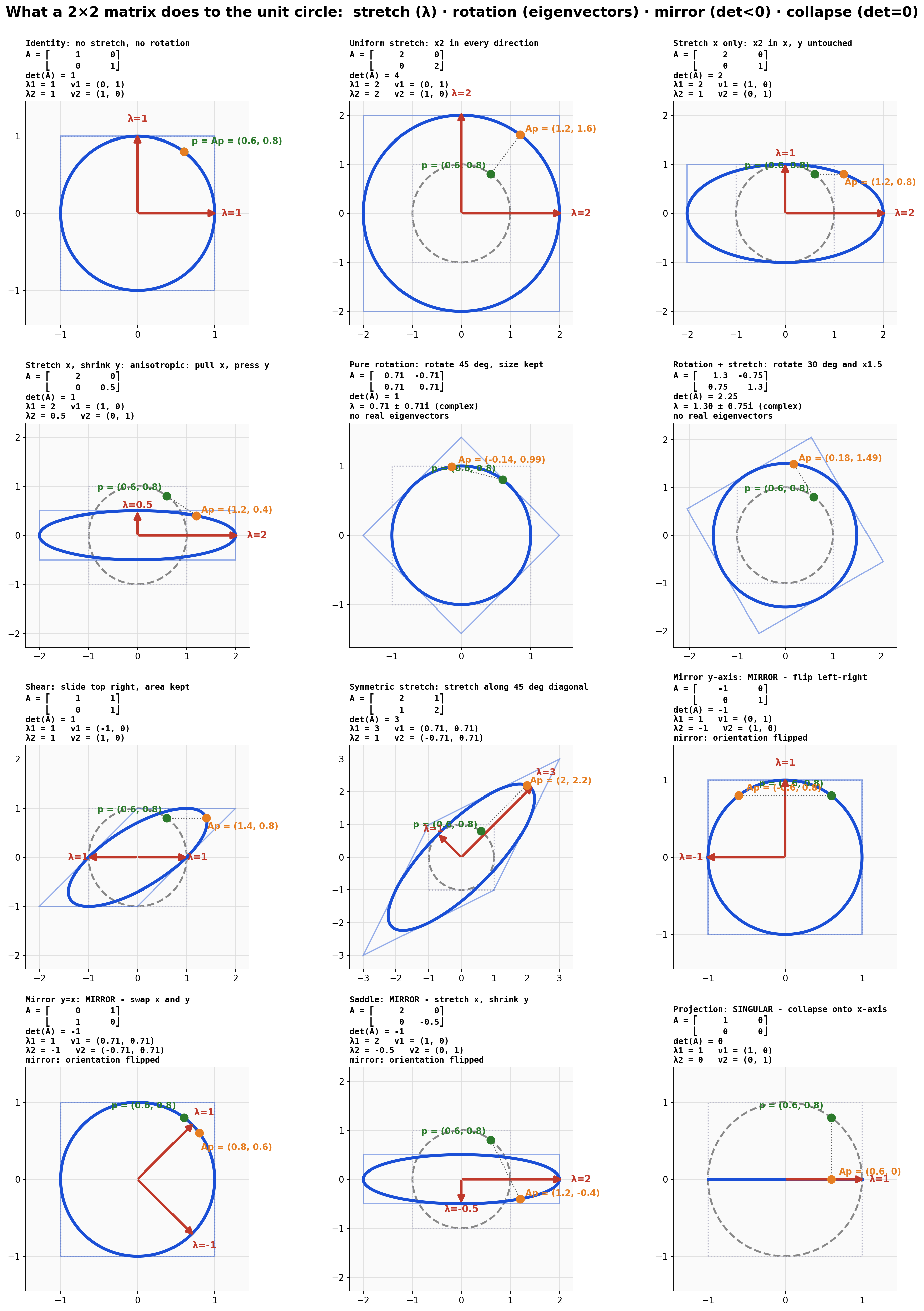
Yes, and it takes exactly one experiment to see it. Take the unit circle – every point whose distance from the origin is one – multiply every single point by the same 2x2 matrix, and look at what shape comes out. That shape IS the matrix. Here is the whole zoo in one gallery, from our teaching notebook:
How to read the gallery
Every panel plays the same game. The dashed gray circle is the input: the unit circle. The solid blue curve is the output: where every point landed after multiplication by the matrix A in the corner. One test point is tracked in every panel: the green dot is p = (0.6, 0.8), and the orange dot is Ap, where it ended up.
The red arrows are the eigenvectors – the special directions that do not rotate, only stretch – and the labels on them are the eigenvalues, the stretch factors along those directions. Keep your eye on two numbers printed in each panel: the eigenvalues and det(A). By the end of this post those two numbers will tell you the whole story.
The five basic moves
Here is every worked multiplication from this post in one place – the same test point p = (0.6, 0.8) pushed through eight different matrices:
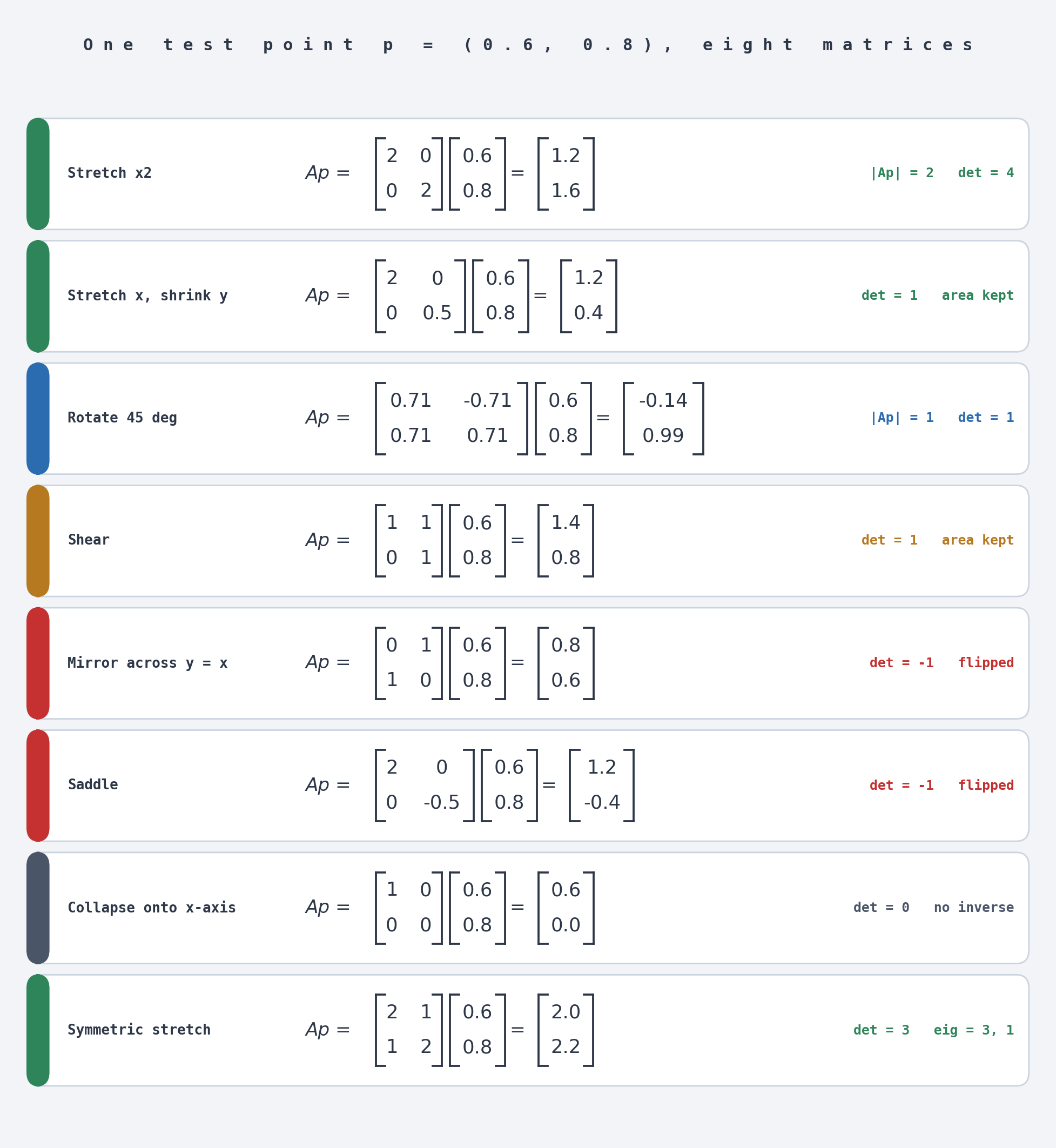
Move 1: stretch. The circle becomes an ellipse. With A = [[2, 0], [0, 2]] every direction doubles (first row of the figure): Ap = (1.2, 1.6), and the length check is
|Ap| = sqrt(1.2^2 + 1.6^2) = sqrt(1.44 + 2.56) = sqrt(4) = 2
The circle is now a circle of radius 2. The eigenvalues are both 2, and the determinant is 4 – the area grew by a factor of 2 x 2 = 4. That is not a coincidence, as we will see below.
Stretching does not have to be fair. With A = [[2, 0], [0, 0.5]] the x direction doubles while the y direction halves: Ap = (1.2, 0.4). The circle flattens into a wide ellipse, and det(A) = 2 x 0.5 = 1 means the total area was preserved even though the shape is unrecognizable.
Move 2: rotate. With A = [[0.71, -0.71], [0.71, 0.71]] – which is [[cos45, -sin45], [sin45, cos45]] rounded – the circle maps onto itself, just turned by 45 degrees: Ap = (0.426 - 0.568, 0.426 + 0.568) = (-0.14, 0.99). Nothing stretched, |Ap| is still 1, and det(A) = 1. Notice the panel says “no real eigenvectors”: a pure rotation moves EVERY direction, so no real vector can keep its direction. The eigenvalues are complex (0.71 + 0.71i and 0.71 - 0.71i) – that is what “this matrix rotates” looks like to the eigenvalue machinery.
Move 3: shear. With A = [[1, 1], [0, 1]] the circle slides into a slanted ellipse, like a deck of cards pushed sideways: Ap = (0.6 + 0.8, 0.8) = (1.4, 0.8). Both eigenvalues are 1 and det(A) = 1: area is preserved, but the shape is distorted. Shear is the reason eigenvalues alone cannot tell you everything – a matrix can have all eigenvalues equal to one and still not be the identity.
Move 4: mirror. With A = [[0, 1], [1, 0]] the coordinates swap: Ap = (0.8, 0.6). Every point on the circle lands on the circle, but the whole picture is flipped across the line y = x. The giveaway is det(A) = -1. A negative determinant always means the same thing: the matrix flipped orientation somewhere, like a mirror or a left hand becoming a right hand. The saddle matrix A = [[2, 0], [0, -0.5]] combines a flip with a stretch: Ap = (1.2, -0.4), and det(A) = -1 as well – the area is preserved, but one axis points the wrong way.
Move 5: collapse. This is the important one. With A = [[1, 0], [0, 0]] the second coordinate is simply deleted: Ap = (0.6, 0.0). The entire circle flattens onto a line segment on the x-axis, and det(A) = 0. The matrix is called singular, and it has no inverse – you cannot un-delete information. A million different points (0.6, anything) all landed on the same spot (0.6, 0), so no operation can tell them apart afterward.
The two cheat codes
After staring at all twelve panels, the pattern is this: you do not need to track every point. Two numbers summarize the whole transformation.
The eigenvectors and eigenvalues tell you the natural axes of the matrix and how much it stretches along them. A vector on an eigen-direction comes out pointing the same way, just scaled by its eigenvalue. That is why the symmetric stretch A = [2, 1], [1, 2] looks so clean once you tilt your head 45 degrees: its eigenvectors are (0.71, 0.71) with eigenvalue 3 and (-0.71, 0.71) with eigenvalue 1, so it is secretly just a “stretch x3 along the diagonal” wearing a disguise. Check on our test point: Ap = (2*0.6 + 1*0.8, 1*0.6 + 2*0.8) = (2.0, 2.2), exactly the orange dot in the gallery.
The determinant tells you what happens to area, and its sign tells you about orientation. A positive determinant means the area scales by det(A) and the orientation is kept. A negative determinant means the area scales by |det(A)| and the orientation is flipped, as with every mirror above. A zero determinant means collapse: a dimension is destroyed and no inverse exists.
And the two cheats are the same cheat: the determinant is the product of the eigenvalues. Uniform stretch: 2 x 2 = 4. Symmetric stretch: 3 x 1 = 3. Mirror: 1 x (-1) = -1. Projection: 1 x 0 = 0.
Why deep learning cares
Every layer of a neural network is a matrix multiply followed by a nonlinearity. When a layer transforms its input, it is doing exactly what these panels show: stretching some directions of the data, compressing others, occasionally rotating, and – if you are unlucky – collapsing. A weight matrix with a tiny determinant is throwing information away. Exploding or vanishing gradients are just these stretch factors compounding over many layers. Once you see a matrix as a machine that warps space, half of linear algebra stops being symbol-pushing and starts being geometry.
One thing to try
Pick any 2x2 matrix and classify it before plotting anything:
import numpy as np

A = np.array([[2, 1],
              [1, 2]])

print(np.linalg.eigvals(A))   # [3. 1.]  stretches x3 and x1
print(np.linalg.det(A))       # 3.0      area triples, no flip
print(np.linalg.eig(A)[1])    # the eigen-directions it stretches along
Then change the 2 in the bottom right to 0.5, watch the determinant go to zero – A is now singular and collapses the plane onto a line – and predict the output shape before you draw it. When your predictions start matching the pictures, you own this material.
The gallery and all arithmetic in this article are adapted from the teaching notebooks I use with my students.
References
- Kneusel, R. T. (2021). Math for Deep Learning: What You Need to Know to Understand Neural Networks. No Starch Press.
- Sanderson, G. (3Blue1Brown). “Eigenvectors and Eigenvalues.” Essence of Linear Algebra, Chapter 14.
I tutor machine learning, deep learning, statistics, and math. If linear algebra – or anything else – is not clicking for you, you can find me on Wyzant.