Distance Metrics: How to measure differences?

Every clustering, nearest-neighbor, and recommendation algorithm depends on one choice you make before anything runs: what the word “close” means. There is no universal answer, because the right ruler depends on the kind of data in front of you, and a bad choice quietly poisons everything that comes after it.

Think about three questions that look unrelated. A bank wants to group customers who behave alike. A doctor wants to know which past patients resemble the one in front of her. A search engine wants documents about the same topic. All three reduce to the same operation: take two rows of a table and produce a number that says how far apart they are. That number is the dissimilarity, and its flip side is the similarity. The catch is that the data never hands you this number. You choose it. Two rows that sit close under one measure can stand far apart under another, and whichever one you pick, the algorithm downstream will carry it out faithfully. Distance is not something you find in the world; it is something you decide. This post walks through the rulers that cover almost every situation, works the arithmetic for each one, and ends with a table for picking between them.

Numeric Data: One Formula with a Dial

When every attribute is a number, the standard tool is the Minkowski distance, and the easiest way to understand it is as one formula with a dial in it. The dial is called h. Take the absolute difference on each attribute, raise each one to the power h, add them up, and take the h-th root. That is the entire family:

d(i,j) = ( |x_i1 - x_j1|^h + |x_i2 - x_j2|^h + ... + |x_ip - x_jp|^h )^(1/h)

Here x_ik is the value of attribute k for object i, and p is the number of attributes. What the dial changes is the shape of a “circle” – the set of points the ruler considers equally far from the center.

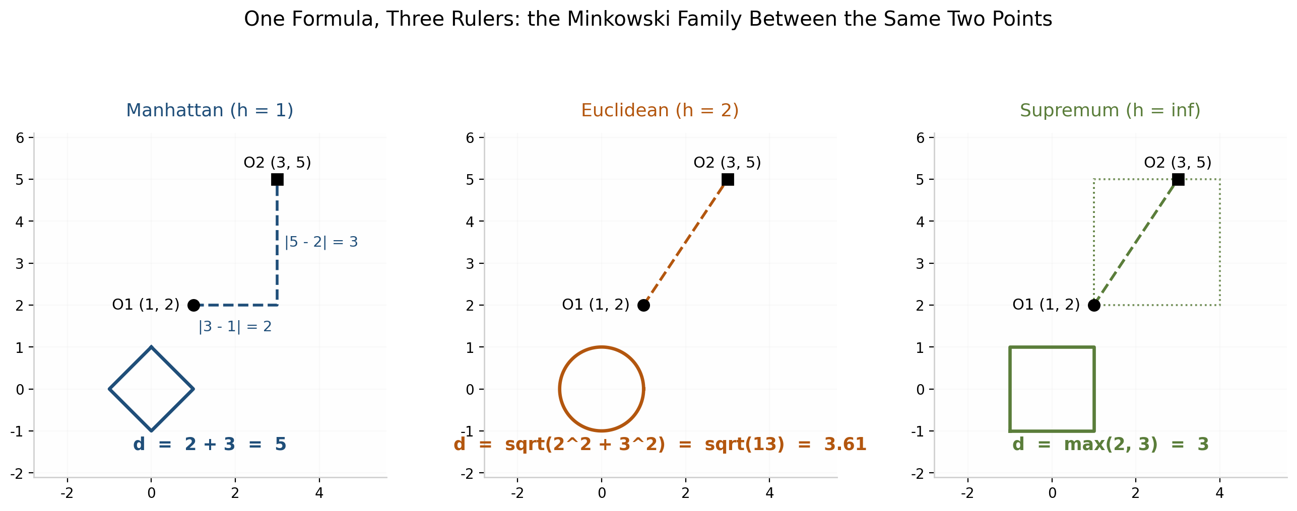
Set h = 1 and you get the Manhattan distance, which travels along the axes like a taxi on a street grid. Between O1 = (1, 2) and O2 = (3, 5), the taxi drives two blocks east and three blocks north, so the distance is 2 + 3 = 5. Set h = 2 and you get the Euclidean distance, the straight line a bird flies: sqrt(2^2 + 3^2) = sqrt(13) = 3.61. Push h to infinity and something curious happens: the biggest single difference swallows all the others, and the distance becomes max(2, 3) = 3. This is called the supremum distance. The figure shows the three unit circles – a diamond, a circle, a square – and the three honest answers for the same pair of points: 5, 3.61, and 3. The dial encodes a belief about how differences should pile up. Manhattan adds them evenly, Euclidean squares them so big ones count more, and the supremum sees nothing but the worst one. Written out separately, the three dial settings are:

Manhattan:  d(i,j) = sum_k |x_ik - x_jk|
Euclidean:  d(i,j) = sqrt( sum_k (x_ik - x_jk)^2 )
Supremum:   d(i,j) = max_k |x_ik - x_jk|

One warning, borrowed from the preprocessing side of the workflow: these rulers take the units as given, so the attribute with the largest scale wins by default. If one column is income in dollars and another is age in years, the distance between two customers is, for all practical purposes, the difference in income. Z-score standardization – subtract the mean, divide by the standard deviation – is what puts the columns on equal footing. This is not housekeeping. It is what makes the comparison fair. And while we are on fine print: a proper distance must be zero only for identical objects (d(i,j) > 0 whenever i != j), it must give the same answer in both directions (d(i,j) = d(j,i)), and the direct route can never be longer than a detour (d(i,j) <= d(i,k) + d(k,j)). A score that passes all three checks is called a metric, and much of clustering theory assumes you are holding one.

Categorical Data: Count the Disagreements

Once the numbers are gone and the attributes are categories – income bracket, zip code, marital status – subtraction means nothing, and the question gets simpler: on what fraction of the attributes do the two objects disagree? Written as a formula, if m of the p attributes match, the distance is simply the fraction of mismatches:

d(i,j) = (p - m) / p

Molly and Greg differ on exactly one of their four attributes, so their distance is ¹⁄₄ = 0.25. The same counting rule covers binary attributes when both outcomes matter equally, which is called the symmetric case. Daniel and Elena, two patients described by six binary test results, differ on one test, so their distance is ¹⁄₆ = 0.17. Counting mismatches sounds crude, but it matches what the data actually holds. Categories have no magnitude, so nothing more precise can honestly be claimed.

Asymmetric Binary: Why “Both Negative” Proves Nothing

Now for the idea that matters most in practice. Look at what Daniel and Elena actually share. Both have a fever, and both tested positive on Test-1 – shared positives, real evidence of similarity. They also share three negatives: neither has a cough, and neither tested positive on Test-3 or Test-4. Should those shared absences count? Medically, no. Two healthy people share thousands of negative test results, and that says nothing about whether they have the same illness. Grocery baskets obey the same logic: the thousands of products two shoppers both skipped tell you nothing about their taste. When presence is rare and meaningful and absence is the boring default – the asymmetric case – the double negatives have to leave the denominator.

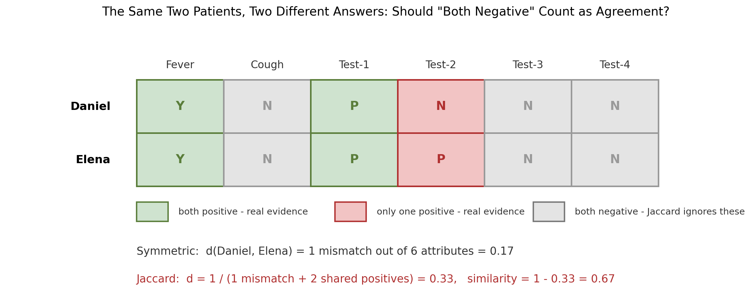
The figure shows both calculations on the same two rows. Count everything, and Daniel and Elena differ on 1 of 6 attributes for a distance of 0.17, which makes them look nearly identical. The Jaccard version keeps only the cells where at least one patient is positive. In the standard notation, q counts the shared positives and r + s counts the mismatches, so the asymmetric distance and its matching similarity are

d(i,j)   = (r + s) / (q + r + s)
sim(i,j) = q / (q + r + s) = 1 - d(i,j)

For Daniel and Elena, q = 2 and r + s = 1: one mismatch plus two shared positives gives three meaningful cells, so d = ¹⁄₃ = 0.33 and the similarity is 1 - 0.33 = 0.67. Same two patients, two answers a factor of two apart, and the asymmetric one is the honest one, because it refuses to treat agreement on nothing as evidence. Choosing the denominator is the whole game here. It is the difference between a recommender that works and one that files everyone who never bought a kayak into the same customer segment.

Ordinal Data: Ranks Become Numbers

Ordinal attributes sit in between. Education level has an order – no_high_school, high_school, college, advanced – but no honest spacing between the rungs. The standard repair takes two steps. First, map each rank onto [0, 1]: if an attribute has M_f distinct ordered values and an object sits at rank r (counting from 1), the converted value is

z = (r - 1) / (M_f - 1)

so the lowest rank gets 0, the highest gets 1, and the rest are spaced proportionally. The four education levels become 0, 0.33, 0.67, and 1, while a three-level income becomes 0, 0.5, and 1. Second, treat the converted values as ordinary numbers and apply any numeric ruler.

The figure shows the mapping for the worked example: O1 = (old, medium, advanced) becomes (1, 0.5, 1), and O2 = (young, low, high_school) becomes (0, 0, 0.33). Reading the three differences off the number lines, the Euclidean distance works out to sqrt((1 - 0)^2 + (0.5 - 0)^2 + (1 - 0.33)^2) = 1.303. One assumption deserves to be said out loud: this encoding claims the rungs are evenly spaced, and in reality college minus high_school is not the same step as advanced minus college. The mapping is a practical device, not a discovery of hidden truth. Its payoff is that ordinal data can now feed every numeric algorithm downstream.

Text and Sparse Vectors: Angles, Not Lengths

Documents, gene profiles, and other long sparse vectors need a different intuition altogether. A document becomes a vector of word counts thousands of entries long, most of them zero. Euclidean distance asks the wrong question in that world, because a long article and a short article on the same topic land far apart simply because one has more words. What carries the topic is the mix of words – the direction the vector points – so the right measure is the cosine of the angle between the two vectors, the dot product divided by the product of the lengths:

cos(d1, d2) = (d1 . d2) / ( ||d1|| * ||d2|| )

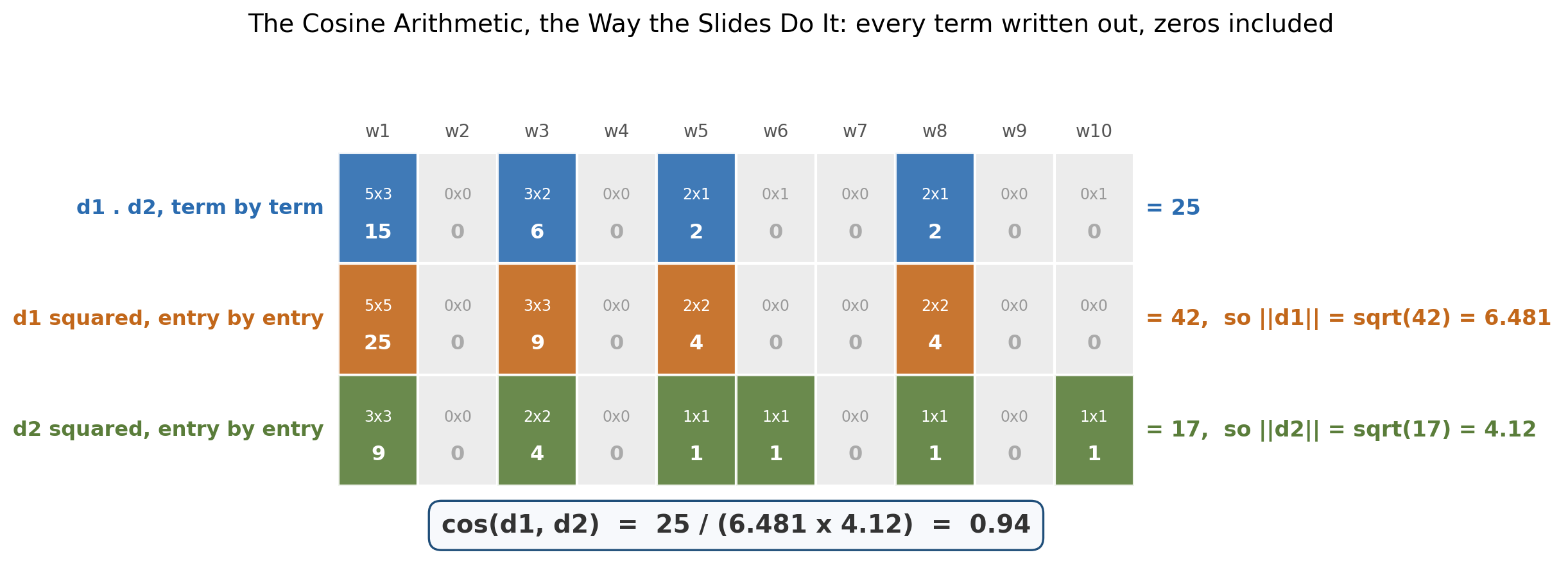
The worked example runs the arithmetic the way the slides do, with all ten terms written out so that nothing hides. The dot product is d1 . d2 = 5*3 + 0*0 + 3*2 + 0*0 + 2*1 + 0*1 + 0*0 + 2*1 + 0*0 + 0*1 = 25, and the figure below shows that only four of the ten word positions contribute anything. The lengths are ||d1|| = (5*5 + 0*0 + 3*3 + 0*0 + 2*2 + 0*0 + 0*0 + 2*2 + 0*0 + 0*0)^0.5 = 42^0.5 = 6.481 and ||d2|| = (3*3 + 0*0 + 2*2 + 0*0 + 1*1 + 1*1 + 0*0 + 1*1 + 0*0 + 1*1)^0.5 = 17^0.5 = 4.12, so cos(d1, d2) = 25 / (6.481 * 4.12) = 0.94. Nearly parallel, which is to say nearly the same document in spirit.

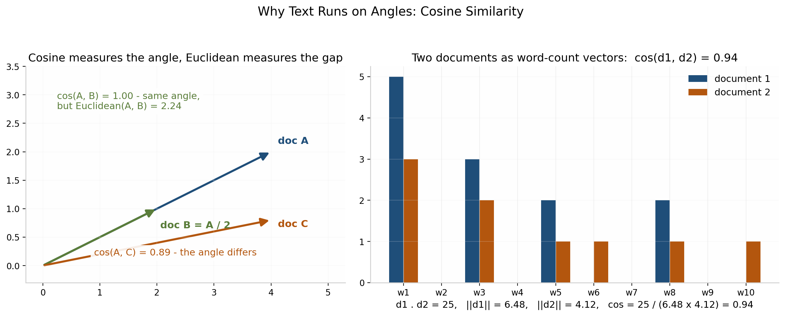
The left panel of the figure shows the property that makes cosine indispensable. Double a vector – the same document written twice as long – and every Euclidean distance involving it changes, while the angle does not move at all, so cos = 1.00 holds exactly. With non-negative counts the cosine sits between 0 and 1, reads 1 for identical directions, and ignores length on purpose. That is why search engines and text clustering think in angles: in long sparse vectors, direction is meaning.

Mixed Types: Gower’s Great Normalizer

Real tables refuse to stay in one lane. A customer record mixes numeric balances, binary flags, categorical channels, and ordinal satisfaction grades in the same row, and no single ruler from above can read the whole thing. Gower’s distance settles the standoff with an idea that is bureaucratic in the best sense: give every attribute its own ruler, force every ruler to report on the common currency of [0, 1], then average – but only over the attributes allowed to vote. Written formally, each attribute f contributes a per-attribute distance d_f in [0, 1] and a vote indicator delta_f that equals 1 when the attribute counts and 0 when it is excluded, and the Gower distance is the average over the voting attributes:

d(i,j) = sum_f( delta_f * d_f ) / sum_f( delta_f )

Numeric attributes contribute their absolute difference divided by the attribute’s range. Categorical and binary attributes contribute 1 on a mismatch and 0 on a match. Asymmetric binary cells where both sides are absent are left out, and so is any attribute with a missing value on either side.

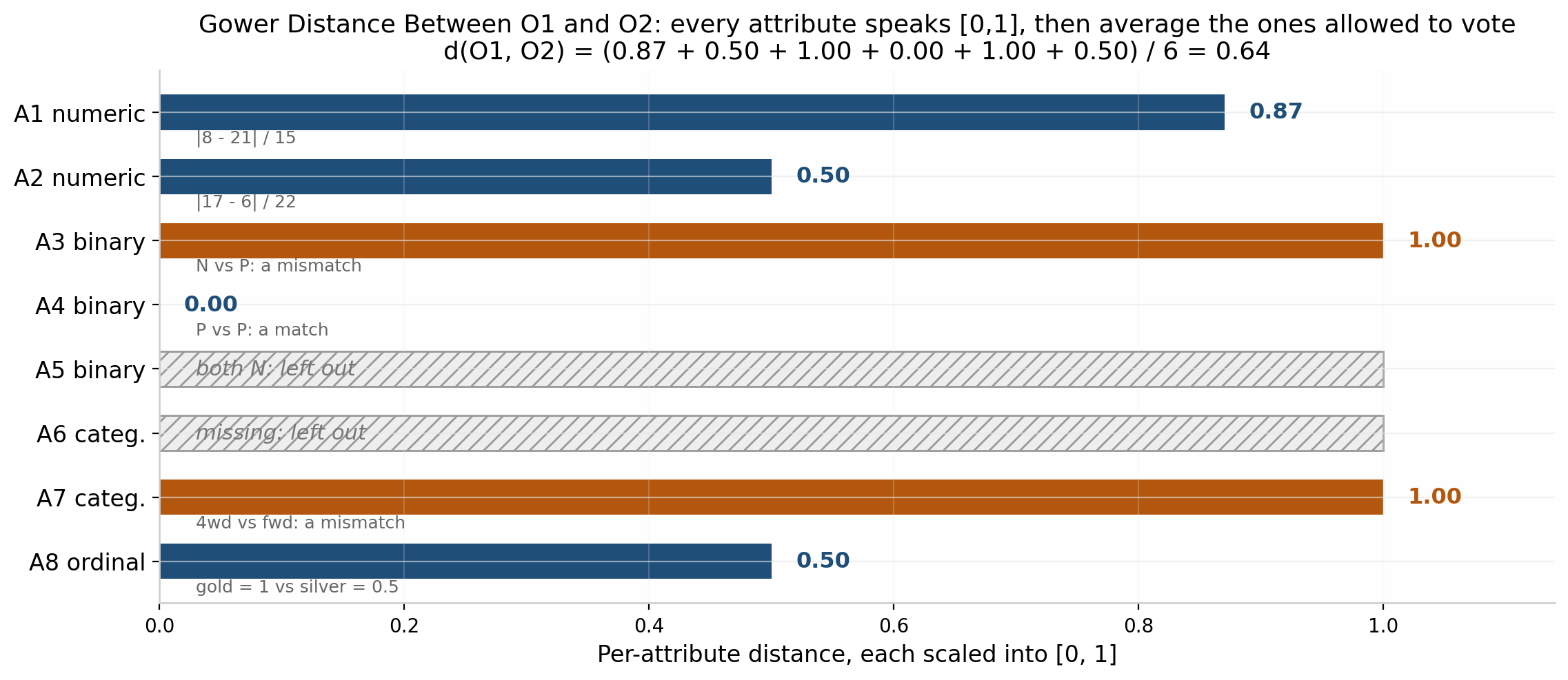
The figure takes the O1-versus-O2 example apart attribute by attribute. The two numeric columns contribute 0.87 and 0.50 after range scaling. The binary columns contribute 1, 0, and one exclusion because both entries were N. The categorical column with a missing value is excluded too. The remaining categorical mismatch contributes 1, and the ordinal medal column – gold mapped to 1, silver to 0.5 – contributes 0.5. Six attributes are left voting, the contributions sum to 3.87, and d(O1, O2) = 3.⁸⁷⁄₆ = 0.64. Notice what the design bought: a dollar column and a yes/no flag both ended up as numbers between 0 and 1, so neither could shout over the other, and the exclusions kept missing data and empty agreement from watering down the verdict.

Choosing the Ruler

The whole topic compresses into one lookup table.

Your attributes look like	Ruler	Watch out for
All numeric, comparable meaning	Minkowski (h = 2 by default)	Standardize first, or the largest scale wins
All numeric, worst case matters	Supremum (h = inf)	One noisy attribute becomes the whole distance
Categories or symmetric binary	Mismatch count	Nothing; it is already as honest as the data allows
Binary where presence is rare	Jaccard	Never let “both absent” into the denominator
Ordered ranks	Map ranks to [0,1], then Euclidean	The equal-spacing assumption is yours, not the data’s
Sparse counts, text, genes	Cosine	It ignores magnitude by design; that is the point
A mix of everything	Gower	Only as good as the per-attribute rulers inside it

Two habits apply no matter which row you pick. First, preprocessing is part of the distance: standardize the numeric columns before you measure, or the units of measurement will choose your clusters for you. Second, the choice is cheap to test. Run the clustering under two plausible rulers and compare the results; if the conclusions flip, the ruler was doing more work than the data, and that is worth knowing. “Similar” is not a property sitting in the world waiting to be measured. It is a modeling decision, and these rulers are the vocabulary you make it in.